The Profile API is a debugging tool that Elasticsearch provides to measure query execution performance. This API breaks down query execution, showing how much time was spent on each phase of the search process. This visibility comes in handy when identifying bottlenecks and comparing different query and index configurations.
In this blog, we will explore how the Profile API can help us compare different approaches to vector search in Elasticsearch, understanding execution times and how the total response time is used across different actions. This showcases how search profiling can drive the settings selection, giving us an example of how each one behaves with a particular use case.
Profile API implementation
Profiler API
To enable search profiling in Elasticsearch, we add a “profile” : ”true” parameter to a search request. This instructs Elasticsearch to collect timing information on the query execution without affecting the actual search results.
For example, a simple text query using profiling:
GET wikipedia-brute-force-1shard/_search
{
  "size": 0,
  "profile": true,
  "query": {
    "match": {
      "text": "semantic search"
    }
  }
}
The main parts of the response are:
"profile": {
    "shards": [
      {
        "id": "[OGMMYXQqRseu_8fR0yD4Qg][wikipedia-brute-force-1shard][0]",
        "node_id": "OGMMYXQqRseu_8fR0yD4Qg",
        "shard_id": 0,
        "index": "wikipedia-brute-force-1shard",
        "cluster": "(local)",
        "searches": [
          {
            "query": [
              {...
            //detailed timing of the query tree executed by Lucene on a particular shard.
               ...
              }
            ],
            "rewrite_time": //All queries in Lucene undergo a "rewriting" process that allows Lucene to perform optimizations, such as removing redundant clauses
            ,
            "collector": [
              {...
             // shows high-level execution details about coordinating the traversal, scoring, and collection of matching documents
               ...
              }
            ]
          }
        ],
        "aggregations": [
             //detailed timing of the aggregation tree executed by a particular shard
        ]
      }
    ]
  }
Kibana profiler
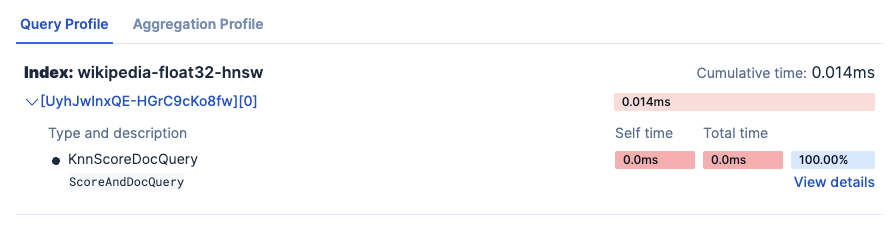
In the DevTools app in Kibana we can find a search profiler feature that makes reading the metrics a lot easier. The search profiler in Kibana uses the same profile API seen above but providing a friendlier visual representation of the profiler output.
You can see how the total query time is being spent:
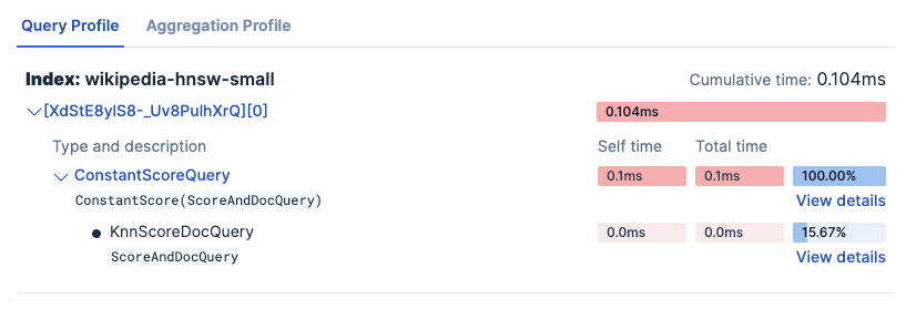
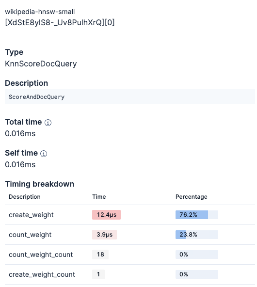
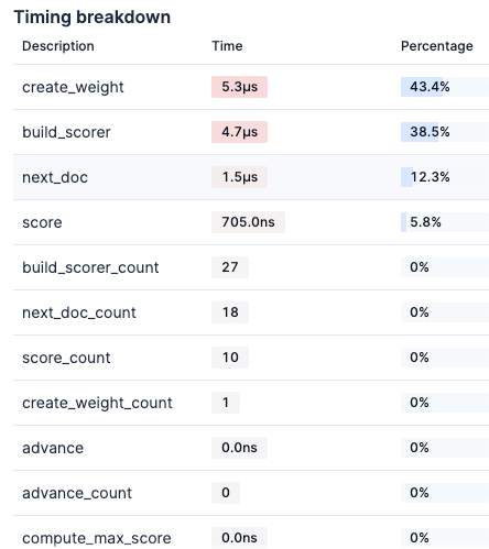
And you can see details on each part of the query.
The profiler feature can help in comparing different queries and index configurations quickly.
When to use the Profile API directly
- Automation: Scripts, monitoring tools, CI/CD pipelines
- Programmatic analysis: Custom parsing and processing of results
- Application integration: Profile directly from your code
- No Kibana access: Environments without a Kibana instance or remote servers
- Batch processing: Profile multiple queries systematically
When to use the search Profiler in Kibana
- Interactive debugging: Quick iteration and experimentation
- Visual analysis: Spot bottlenecks through color coding and hierarchy views
- Collaboration: Share visual results with other people
- Ad-hoc investigation: One-off performance checks without coding
Basic profiling KNN example
For a simple KNN search, we can use:
GET wikipedia-brute-force-1shard/_search
{
  "query": {
    "bool": {
      "must": [
        {
          "knn": {
            "field": "embedding",
            "query_vector": [...],
            "k": 10,
            "num_candidates": 1500
          }
        },
        {
          "match": {
            "text": "country"
          }
        }
      ],
      "filter": {
        "term": {
          "category": "medium"
        }
      }
    }
  },
  "size": 10,
  "_source": [],
  "profile": true
}
Main KNN search metrics in Elasticsearch
We can find KNN metrics in the dfs section of the profile. It shows the execution time for query, rewrite, and collector phases; it also shows the number of vector operations executed in the query.
Vector search time (rewrite_time)
This is the core metric for vector similarity computation time. In the profile object, it's found at:
"dfs": {
  "knn": [{
    "rewrite_time": 198703  // nanoseconds
  }]
}
Unlike traditional Elasticsearch queries, kNN search performs the bulk of its computational work during the query rewrite phase. This is a fundamental architectural difference.
The rewrite_time value represents the cumulative time spent on Vector similarity calculations, HNSW graph traversal and Candidate evaluation
Vector operations count
Found in the same KNN section:
"vector_operations_count": 15000This metric tells you how many actual vector similarity calculations were performed during the kNN search.
Understanding the count
In our query with num_candidates: 1500, the vector operations count represents:
- Approximate search efficiency: The number of vectors actually compared during HNSW (Hierarchical Navigable Small World) graph traversal
- Search accuracy trade-off: Higher counts mean a more thorough search, but longer execution time
Query processing time (time_in_nanos)
After finding vector candidates, Elasticsearch processes the actual query on this reduced set:
"query": [{
"type": "BooleanQuery",
"description": "+DenseVectorQuery.Floats +text:country #category:medium",
"time_in_nanos": 5064686,
"children": [
{
"type": "Floats",
"description": "DenseVectorQuery.Floats",
"time_in_nanos": 566195
},
{
"type": "TermQuery",
"description":
"text:country",
"time_in_nanos": 667083
},
{
"type": "TermQuery",
"description": "category:medium",
"time_in_nanos": 2725249
}
]
}]
The time_in_nanos metric covers the query phase: the computational work of finding and scoring relevant documents. This total time is broken down into children, and each child query represents a clause in our Boolean query:
DenseVectorQuery
- Processing kNN results: Scoring the candidate documents identified by kNN
- Not computing vectors: Vector similarities were already computed in DFS phase
- Fast because: Operating only on the pre-filtered candidate set (10-1500 docs, not millions)
TermQuery: text:country
- Inverted index lookup: Finding documents containing "country"
- Posting list traversal: Iterating through matching documents
- Term frequency scoring: Computing BM25 scores for matched terms
TermQuery: category:medium
- Filter application: Identifying documents with category="medium"
- No scoring needed: Filters don't contribute to score (notice
score_count: 0)
Collection time
The time spent collecting and ranking results:
"collector": [{
  "name": "QueryPhaseCollector",
  "reason": "search_query_phase",
  "time_in_nanos": 270704,  // ~271 microseconds
  "children": [
    {
      "name": "TopScoreDocCollector",
      "reason": "search_top_hits",
      "time_in_nanos": 215204  // ~215 microseconds
    }
  ]
}]
The time_in_nanos for collectors breaks down into:
TopScoreDocCollector
- Collects top hits from the query results.
Understanding collection in Elasticsearch's architecture
In Elasticsearch, a query is distributed among all relevant shards, where it is executed individually. The collection phase operates across Elasticsearch's distributed shard architecture like this:
Per-Shard Collection: Each shard collects its top-scoring documents using the TopScoreDocCollector. This happens in parallel across all shards that hold relevant data.
Result Ranking and Merging: The coordinating node (the node that receives your query) then receives the top results from each shard and merges these partial results together by score to find the global top N results
So for our example:
QueryPhaseCollector (270μs): The time spent on the query phase collection within a single shard.
TopScoreDocCollector (215μs): The actual time spent collecting and ranking top hits from that shard
Note that these times represent the collection phase on a single shard in the profile output. For multi-shard indices, this process happens in parallel on each shard, and the coordinating node adds additional overhead for merging and global ranking, but this merge time is not included in the per-shard collector times shown in the Profiler API.
Experiment set up
The script consists of running 50 queries per experiment using the Profiler under four experiment setups. The experiments measure query processing, fetch, collection, and vector search execution times across multiple index configurations with different vector indexing strategies, quantization techniques, and infrastructure setups:
- Experiment 1: Comparing query performance on a flat dense vector vs a HNSW quantized dense vector.
- Experiment 2: Understanding the effect of oversharding in vector search.
- Experiment 3: Understanding how Elastic boosts the performance of a vector query with filters by applying them before the more expensive KNN algorithm.
- Experiment 4: Comparing the performance of a cold query vs a cached query.
Getting started
Prerequisites
- Python 3.x
- An Elasticsearch deployment
- Libraries
- Elasticsearch
- Pandas
- Numpy
- Matplotlib
- Datasets (HuggingFace library)
To reproduce this experiment, you can follow these steps:
1. Clone the repository
git clone https://github.com/Alex1795/profiler_experiments_blog.git2. Install required libraries:
pip install -r requirements.txt3. Run the upload script. Make sure to have the following environment variables set beforehand
- ES_HOST
- API_KEY
Example configuration:
ES_HOST="<your_deployment_url>"
API_KEY="<your_api_key>"
To run the upload script, use:
python data_upload.pyThis might take several minutes; it is streaming the data from Hugging Face.
4. Once the data is indexed in Elastic, you can run the experiments using:
python profiler_experiments.pyDataset selection
For this analysis, we will be using pre-generated embeddings generated from the wikimedia/wikipedia dataset, created using the Qwen/Qwen3-Embedding-4B model. We can find these embeddings already generated in Hugging Face.
The model produces 2560-dimensional embeddings that capture the semantic relationships in the Wikipedia articles. This makes this dataset an adequate candidate for testing vector search performance with different index configurations. We will take 50.000 datapoints (documents) from the dataset.
All the documents will be used in 4 indices with 4 different configurations for the dense_vector field.
Profiler data extraction
The heart of the experiments is the extract_profile_data method. This function gets these metrics from the response:
| Original field in the Search Profile | Extracted metric | comment |
|---|---|---|
| response['took'] | total_time_ms | The total time the query took to execute, populated directly from the top-level 'took' key. |
| shard['dfs']['knn'][0]['rewrite_time'] | vector_search_time_ms | The total time spent on vector search operations across all shards, aggregated and converted from nanoseconds to milliseconds. |
| shard['dfs']['knn'][0]['vector_operations_count'] | vector_ops_count | The total number of vector operations performed during the search, aggregated across all shards. |
| shard['searches'][0]['query'][0]['time_in_nanos'] | query_time_ms | The total time spent on query execution across all shards, aggregated and converted from nanoseconds to milliseconds. |
| shard['searches'][0]['collector'][0]['time_in_nanos'] | collect_time_ms | The total time spent on collecting and ranking results across all shards, aggregated and converted from nanoseconds to milliseconds. |
| shard['fetch']['time_in_nanos'] | fetch_time_ms | The total time spent on retrieving documents across all shards, aggregated and converted from nanoseconds to milliseconds. |
| len(response['profile']['shards']) | shard_count | The total number of shards the query was executed on. |
| (Calculated) | other_time_ms | The remaining time after accounting for vector search, query, collect, and fetch times, representing overhead such as network latency. |
Indices configuration
Each index will have 4 fields:
- text (text type): The original text used to generate the embedding
- embedding (dense_vector type): 2560-dimensional embedding with a different configuration for each index
- category (keyword type): A classification of the length of the text short, medium or long
- text_length (integer type): Words count of the text
Relevant settings:
- Embedding type: float
- Number of shards: 1
Relevant settings:
- Embedding type: float
- Number of shards: 3
Relevant settings:
- Embedding type: HNSW
- m=16 (The number of neighbors each node will be connected to in the HNSW graph)
- ef_construction=200 (The number of candidates to track while assembling the list of nearest neighbors for each new node)
To learn more about parameters for the dense vector field, see: Parameters for dense vector fields
Experiment execution
Experiment 1: Flat vs int 8 HNSW dense vector
Objective: Compare the performance of a flat dense vector against a vector using HNSW.
Indices to use:
- wikipedia-brute-force-1shard
- wikipedia-int8-hnsw
Hypothesis: The HNSW index will have significantly lower query latency, especially on larger datasets, as it reduces memory usage by 75% and it avoids comparing the query vector with each vector in the dataset.
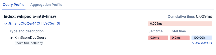
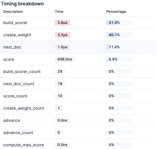
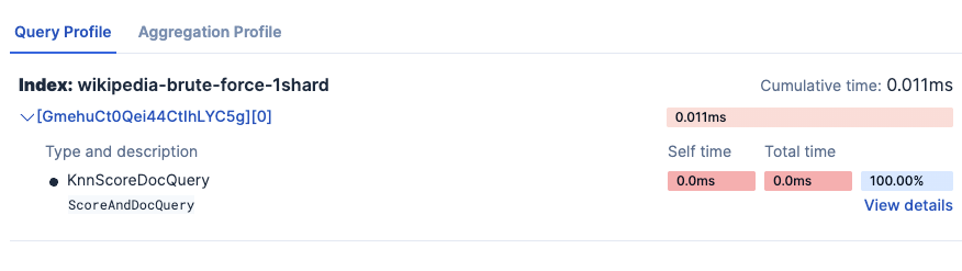
Kibana Search Profiler results:
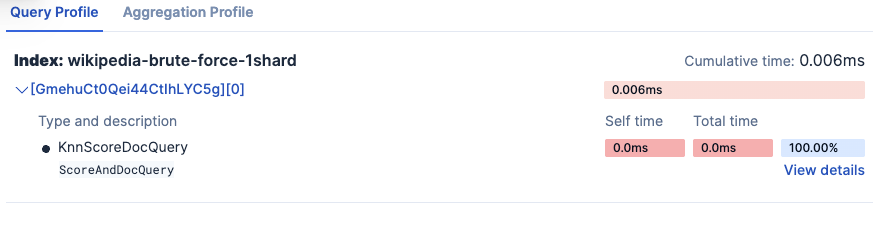
- wikipedia-brute-force-1shard
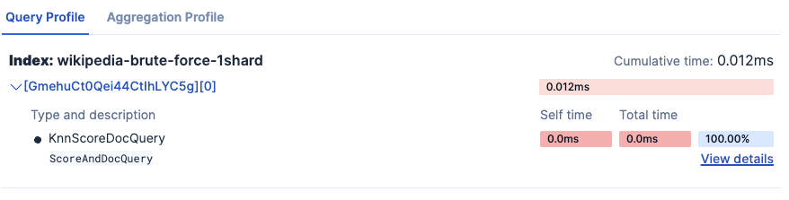
- wikipedia-int8-hnsw
Experiment results:
=== Experiment 1: Flat vs. HNSW dense vector ===
Testing Flat (float32) (wikipedia-brute-force-1shard)...
Average total time (ES): 528.67ms
Average vector search time: 517.52ms
Average query time: 0.01ms
Average collect time: 0.01ms
Average fetch time: 7.37ms
Average wall clock time: 853.63ms
Vector operations: 50000
Testing HNSW (int8) (wikipedia-int8-hnsw)...
Average total time (ES): 12.67ms
Average vector search time: 3.66ms
Average query time: 0.01ms
Average collect time: 0.01ms
Average fetch time: 7.47ms
Average wall clock time: 140.74ms
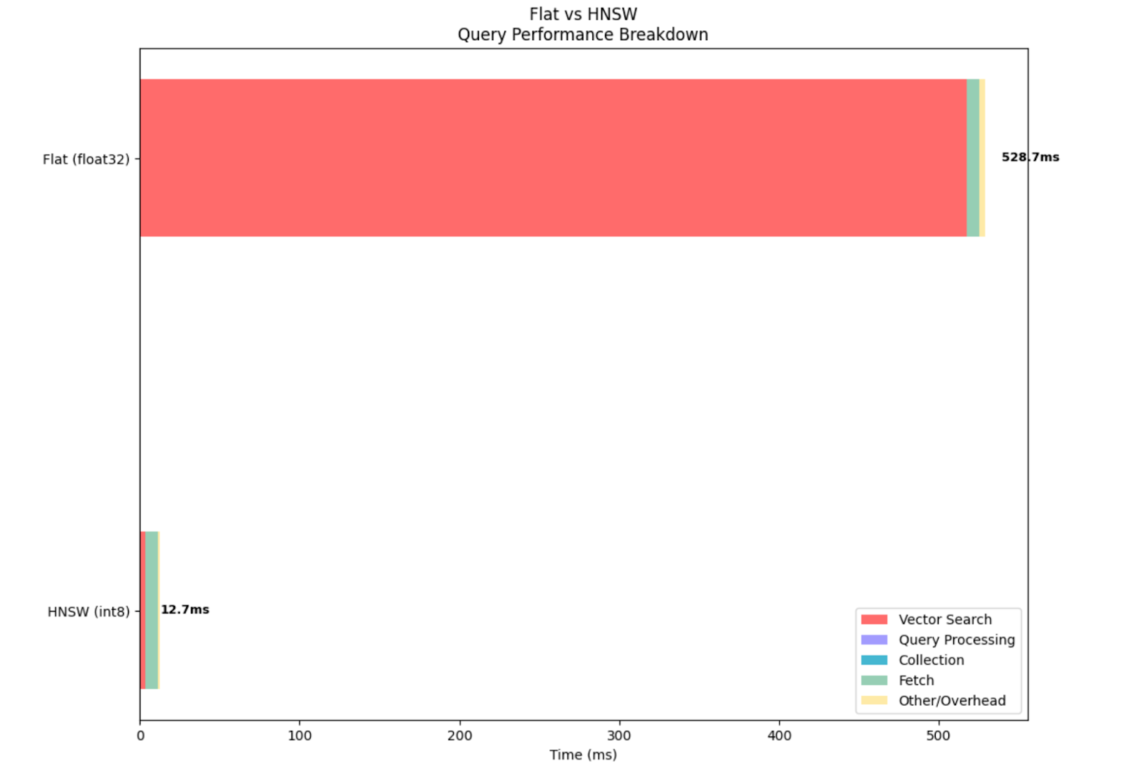
Vector operations: 2352We can see from the metrics that the float approach did 50000 vector operations, which means it compared the query vector with each vector in the dataset, which resulted in ~140 times increase in the vector search time when compared with the HNSW vector.
From the graph below, we can visualize that even if other metrics are similar, the Vector search takes much longer with a float-type dense vector. That being said, it is worth noting that BBQ quantization reduces the recall when compared with a non-quantized vector.
Experiment 2: Impact of over-sharding on brute force search
Objective: Understand how excessive sharding on a single-node Elasticsearch deployment negatively impacts vector search query performance
Indices to use:
- wikipedia-brute-force-1shard: The single-shard baseline.
- wikipedia-brute-force-3shards: The multi-shard version.
Hypothesis: On a single-node deployment, increasing the number of shards will degrade query performance rather than improve it. The 3-shard index will exhibit higher total query latency compared to the 1-shard index. This can be extrapolated to having an inadequate number of shards for our infrastructure.
Kibana Search Profiler results:
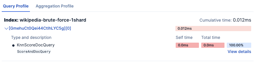
- wikipedia-brute-force-1shard
- wikipedia-brute-force-3shards
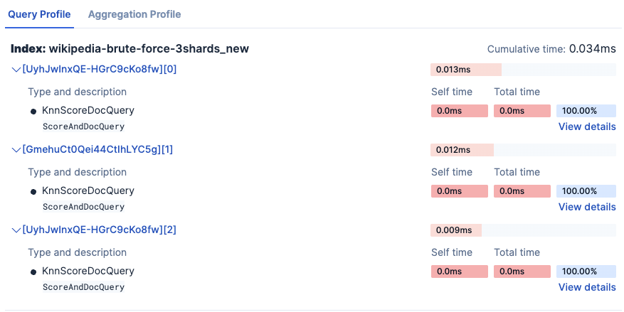
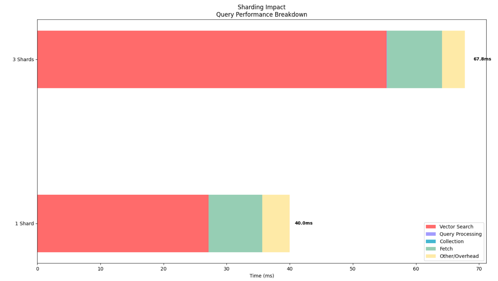
Notice time is more than 3 times here because it runs in 3 separate shards.
Experiment results:
=== Experiment 2: Impact of Sharding on Brute Force Search ===

Testing 1 Shard (wikipedia-brute-force-1shard)...
  Shards: 1
  Average total time (ES): 40.00ms
  Average vector search time: 27.15ms
  Average query time: 0.01ms
  Average collect time: 0.01ms
  Average fetch time: 8.50ms
  Average wall clock time: 204.40ms
  Vector operations: 50000

Testing 3 Shards (wikipedia-brute-force-3shards)...
  Shards: 3
  Average total time (ES): 67.77ms
  Average vector search time: 55.36ms
  Average query time: 0.02ms
  Average collect time: 0.03ms
  Average fetch time: 8.70ms
  Average wall clock time: 338.77ms
  Vector operations: 50000
We can see that even when executing the exact same number of vector operations, having too many shards for this specific dataset added more vector search time, overall making the query slower. This demonstrates how our sharding strategy must go hand in hand with our cluster architecture.
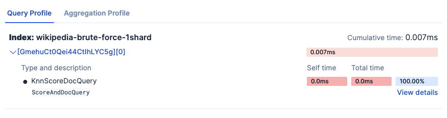
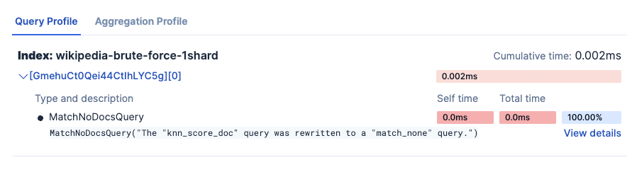
Experiment 3: Combined filter and vector search
Objective: Demonstrate how Elasticsearch efficiently handles pre-filtering before a vector search.
Indices to use:
- wikipedia-brute-force-1shard
Note: This experiment is only applicable to hosted deployments, since we can't control the number of shards on serverless. It will be automatically skipped in a serverless project.
Setup: Construct a query that combines a KNN query for a vector search with a filter.
Hypothesis: When a filter is applied, Elasticsearch first prunes the documents that don't match the filter before performing the expensive vector search on the matching documents. The Profile API will show that the number of documents searched by the vector search operation is significantly lower than the total number of documents in the index, leading to a faster query.We will run the query with 4 configurations:
"knn": {
        "field": "embedding",
        "query_vector":[...],
        "k": k,
        "num_candidates": num_candidates,
        "filter":[] // no filters
}
- Term filter on the category field
"knn": {
        "field": "embedding",
        "query_vector":[...],
        "k": k,
        "num_candidates": num_candidates,
        "filter":[
          {
            "term":{
              "category": "short" // term filter on category
               }
          }
         ]
}
- Range filter on the text_length field
"knn": {
        "field": "embedding",
        "query_vector":[...],
        "k": k,
        "num_candidates": num_candidates,
        "filter":[
          {
            "range":{
              "text_length": { // range filter on text_length
 			"gte": 1000,
"lte": 2000
}
               }
          }
         ]
}
- A combined filter: term filter on the category field + range filter on the text_length field
"knn": {
        "field": "embedding",
        "query_vector":[...],
        "k": k,
        "num_candidates": num_candidates,
        "filter":[ // the two previous filters combined in the same query
          {
            "range":{
              "text_length": {
 			"gte": 1000,
"lte": 2000
}
               }
          },
	   {
            "term":{
              "category": "short"
               }
          }
         ]
}
Results:
=== Experiment 3: Combined Filter and Vector Search ===

Testing No Filter...
  Total hits: 10.0
  Average total time (ES): 50.80ms
  Average vector search time: 42.37ms
  Average query time: 0.01ms
  Average collect time: 0.01ms
  Average fetch time: 7.07ms
  Average wall clock time: 287.01ms
  Vector operations: 50000

Testing Category Filter...
  Total hits: 10.0
  Average total time (ES): 8.00ms
  Average vector search time: 0.78ms
  Average query time: 0.01ms
  Average collect time: 0.01ms
  Average fetch time: 6.11ms
  Average wall clock time: 134.40ms
  Vector operations: 198

Testing Text Length Filter...
  Total hits: 10.0
  Average total time (ES): 18.40ms
  Average vector search time: 9.93ms
  Average query time: 0.01ms
  Average collect time: 0.02ms
  Average fetch time: 7.15ms
  Average wall clock time: 144.74ms
  Vector operations: 10387

Testing Combined Filters...
  Total hits: 1.0
  Average total time (ES): 2.20ms
  Average vector search time: 0.68ms
  Average query time: 0.00ms
  Average collect time: 0.01ms
  Average fetch time: 0.59ms
  Average wall clock time: 127.28ms
  Vector operations: 1
We can see that applying filters adds fetch time to our search, but in exchange, it reduces the vector search time dramatically because it executes less vector operations. This shows how Elastic handles filtering before vector search to improve performance and avoid wasting resources by running the vector search before filtering out irrelevant documents.
Even if the results are constrained to a maximum (k=10), underneath, more vector operations are being executed if we don't filter out some documents before. This effect is more notorious with a flat dense vector, of course, but even in quantized vectors, we can still reduce execution time by applying filters before the vector search.
In the graph, we can see how the query time increased with the filters, but the vector search time is much lower, resulting in lower times overall. We can also see that having more filters impacted the time positively (meaning it lowered the total time), so actually applying the filters is worth it, as the overall time decreases.
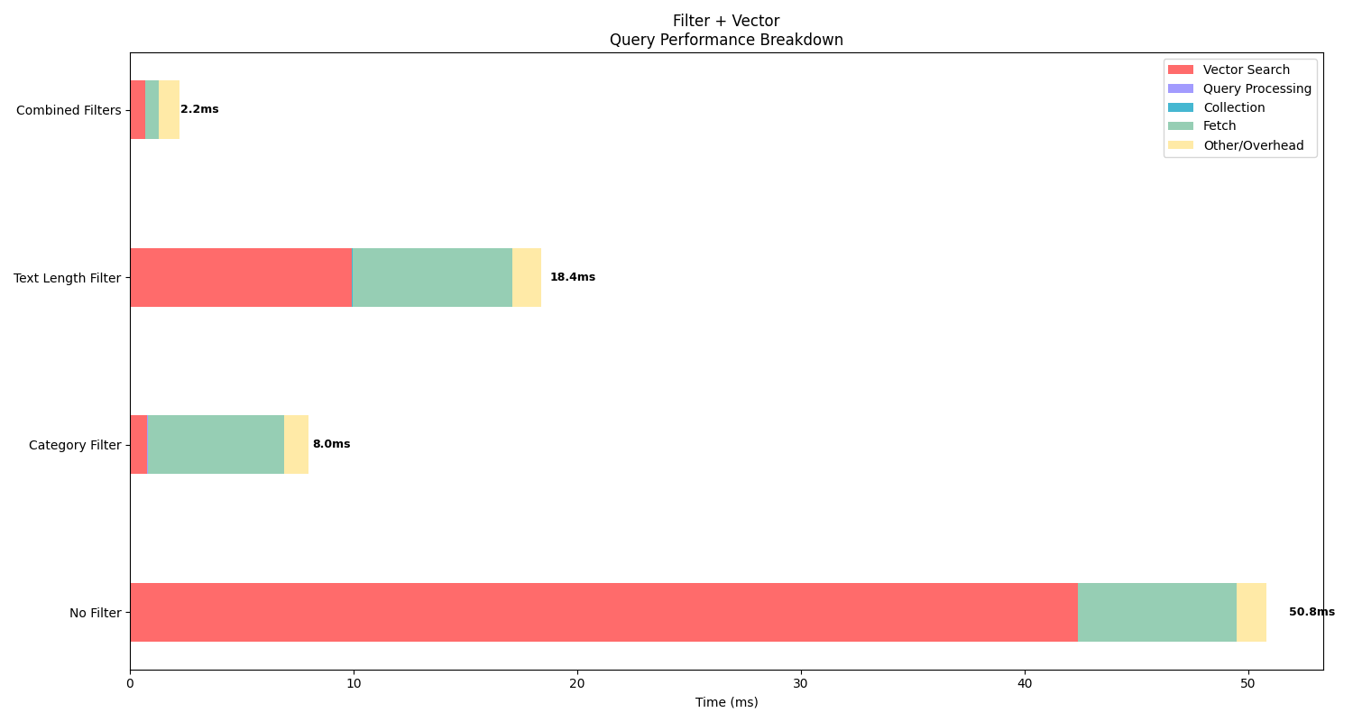
The results highlight how filtering improves efficiency and is a key benefit of using a hybrid search engine like Elasticsearch.
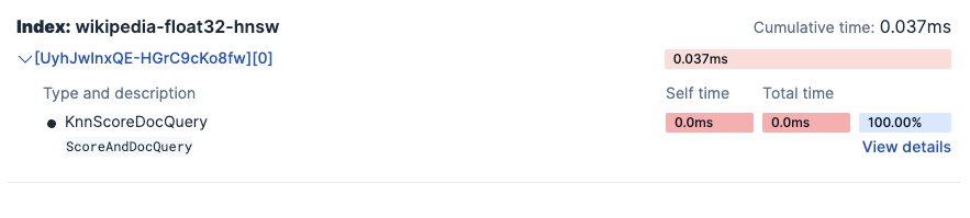
Experiment 4: Compare cold vs cached query performance
Objective: Demonstrate how Elasticsearch's caching mechanisms significantly improve query performance when the same vector search is executed multiple times.
Indices to use:
- wikipedia-float32-hnsw
Setup:
First, clear the Elasticsearch cache
Execute the same vector search query twice:
- Cold query: First execution after cache clearing
- Cached Query: Second execution with caches populated
Hypothesis:The cached (warm) query will execute significantly faster than the cold query. The Profile API will show reduced times across all query phases, with the most dramatic improvements in vector search operations and data retrieval phases.
Results:
=== Experiment 4: Cache Performance (Cold vs Warm Queries) ===
Testing Cold Query (First Run)...
Clearing caches...
Runs executed: 1
Average total time (ES): 490.00ms
Average vector search time: 474.77ms
Average query time: 0.01ms
Average collect time: 0.01ms
Average fetch time: 13.48ms
Average wall clock time: 728.77ms
↳ This represents cold start performance
Testing Warm Query (Cached)...
Runs executed: 5
Average total time (ES): 14.60ms
Average vector search time: 6.99ms
Average query time: 0.01ms
Average collect time: 0.01ms
Average fetch time: 3.96ms
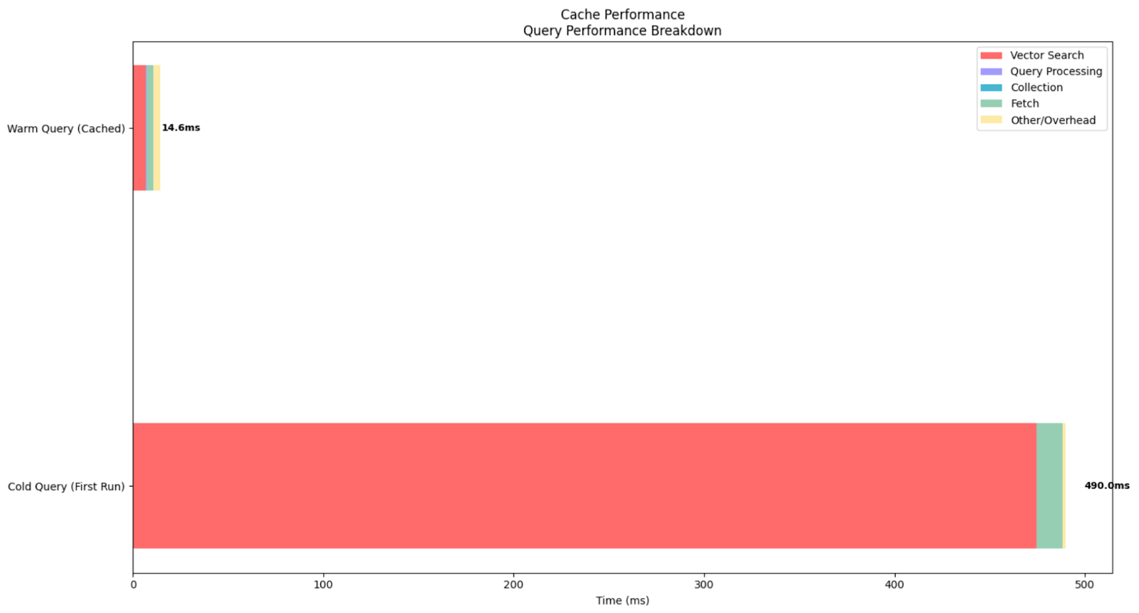
Average wall clock time: 144.35msThis experiment shows the impact of Elasticsearch's cache on vector search performance. Elastic keeps the embedding data in memory, so it executes faster. On the other hand, if the data isn’t in memory and Elastic has to read from disk often, searches become slower.
In this case, the cold query, executed after clearing all caches, took 490ms total time with vector search operations consuming 474.77ms. This shows the "first-time" cost of loading index segments and vector data structures into memory. In contrast, the warm queries averaged just 14.6ms total time with vector search dropping to 6.99ms, demonstrating a remarkable 33x overall speedup and 68x improvement in vector search operations.
In the graph, we can see the huge difference between the cached and cold queries. This result highlights why vector search systems benefit from an initial warm-up period.
Conclusion
Search profiling can let us look into the execution of our queries and, by extension, compare them. This opens the door to comprehensive analysis that can drive design decisions. In our particular experiment, we could see the difference between dense vector configurations and derive complex insights.
Particularly, in our experiments, we have been able to use the profiler to confirm in practice that:
- A quantized dense vector performs queries much faster than a non-quantized one
- Having an appropriate sharding strategy can lead to better performance
- Combining vector search + filters is a powerful tool to improve performance in our queries
Cache can impact performance meaningfully, so for production systems, it might be a good idea to start with a warm-up process using common queries.
Ready to try this out on your own? Start a free trial.
Elasticsearch has integrations for tools from LangChain, Cohere and more. Join our advanced semantic search webinar to build your next GenAI app!
Related content

May 27, 2026
Cutting Elasticsearch DiskBBQ query quantization time by 5x
See how asymmetric quantization cuts DiskBBQ query quantization overhead from about 20% to 4% with little recall impact.
May 28, 2026
How we doubled vector search throughput on Elasticsearch Serverless
How we brought Elasticsearch's native SIMD scoring engine to serverless, and why serverless is where vector search innovation happens next.
May 19, 2026
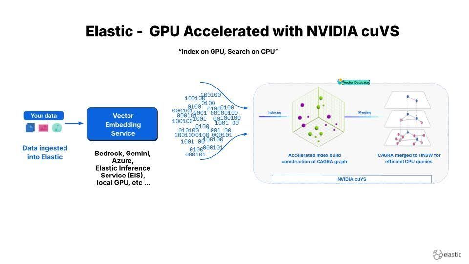
12x faster Elasticsearch vector indexing: deploying NVIDIA cuVS with GPU and CPU tiers
Two patterns for deploying NVIDIA cuVS GPU-accelerated HNSW indexing in Elasticsearch: combined build-and-serve nodes for small clusters and a dedicated GPU ingest tier with ILM handoff to CPU for production at scale.

May 21, 2026
Up to 3x faster stored-vector queries in Elasticsearch
Elasticsearch 9.4 provides a simpler way to search with vectors stored in an Elasticsearch index, with up to 3x lower latency.

May 13, 2026
Elasticsearch Vector DiskBBQ filter search is now 3–5x faster
Learn how Elasticsearch 9.4 makes restrictive filtered DiskBBQ vector search 3–5x faster and more stable by avoiding wasted centroid and postings-list work when selectivity is high.